NATIONAL LAND COVER DATASET

Produced by the USGS, National Land Cover Dataset (NLCD) is available for the 48 contiguous states at 30-meter resolution (Figure 9). It derives from Landsat Thematic Mapper imagery taken during the early to mid 1990s with 1992 as the oldest collection date. Coverage ends abruptly at the borders with Canada and Mexico and seaward at the 12 nautical-mile limit of US territorial waters.

NLCD is a type of categorical land cover data, which is the most common variety of raster land cover data available. With categorical land cover data, each pixel represents a sampled area on the ground and receives a classification as one type of land cover or another. For example, if the contents of a 30 x 30-meter sample of NLCD were 51 percent shrub and 49 percent evergreen forest, then the sample receives the shrub assignation entirely—the winner takes all. What categorical land cover lacks in subtlety, it makes up for in quantity. The millions of pixels that comprise these data when reduced in scale blend land cover colors together smoothly, a desirable trait on natural-color maps. The effect is much like Shelton’s airbrush technique of spraying atomized color droplets.

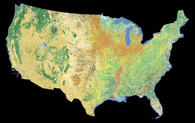
Figure 9. NCLD mosaic of the 48-contiguous states, using the USGS suggested color scheme.

NLCD uses a modified form of the USGS’s Anderson Land Use and Land Cover Classification System (Anderson et al., 1972). The full Anderson classification system consists of four hierarchical levels and more than one hundred categories of land cover (occupying the two uppermost levels) and land use (occupying the two bottommost levels). The distinction between land cover and land use is an important one. For example, forest is a land cover category and bird watching or fire wood collecting are uses that occur in a forest. Because determining detailed land use information is impossible on a national dataset made from 30-meter-resolution Landsat imagery, the NLCD classification does away with land use altogether. It instead consists of a two-level system with nine level-one land cover categories and 21 level-two categories (Figure 10, left).

The USGS developed NLCD for scientific and analytical tasks. Therefore, to make natural-color maps, which are at heart artistic products, requires a change in thinking about what the NLCD classification does. Taking a cue again from Shelton, we next will transform the scientific NLCD classification into an artist’s color palette (figure 10, right).

Figure 10. (left) The NLCD classification with USGS assigned colors. (right). The derivative color palette used for natural-color mapping.

From classification to palette

The first step was reducing NLCD categories from 21 to 15 so as not to overwhelm the reader with too much information. Because every pixel is accounted for with categorical land cover data, reducing the number of NLCD categories required methods other than simple deletion to avoid the appearance of null areas on the final map.

Aggregation, a method that combines several categories as a single generic category, was the method most commonly used. For example, cropland in the color palette represents the aggregation of row crops, small grains, and fallow from the NLCD classification. These detailed and temporally sensitive agricultural categories do not contribute to our geographic understanding on a small-scale map of the US. Reclassification was another helpful method. For example, the NLCD category transitional mostly represents clear-cut and burned forestlands in the western US. Working under the optimistic assumption that the trees will eventually grow back, the palette reclassifies and groups transitional with evergreen forest. Similarly, the NLCD category urban/recreational grasses represent golf courses, schoolyards, and other open areas found in urban environments. Reclassifying this as low intensity development in the palette rather than as a subset of herbaceous planted/cultivated gave discontinuous urban areas on the final map a more concentrated appearance.

The transformation of NLCD into a palette also required the creation of new categories. On natural-color maps the appearance of white (snow) in lofty mountain areas tells readers that these areas are higher and colder than adjacent lowlands. In the continental US, however, the NLCD category perennial ice/snow occupies only scattered tiny areas in the Cascades and northern Rockies. To give high western mountains the emphasis they deserve, the palette contains a new category called alpine. It encompasses all areas above timberline and slightly lower in select places, such as the snowy and rugged Wasatch Range of Utah that barely reaches timberline. Because the elevation of timberline varies depending on latitude, continentality, and other factors, a DEM and biogeography references proved essential for delineating alpine areas. The procedure involved reclassifying all perennial ice/snow, barren, shrubland, and herbaceous/grassland as alpine for areas above the documented timberline elevation of each mountain range (Arno and Hammerly, 1984).

Another new palette category was desert southwest shrub. In the NLCD classification shrubland is the largest single category, representing 18 percent of the total area of the continental US and dominating vast tracts of the intermountain West to the exclusion of all else. The creation of the desert southwest shrub category recognizes that not all shrublands are the same and brings needed graphical variation to these otherwise monotonous regions. Using a DEM to subdivide the shrubland category by elevation zone, desert southwest shrub, which is depicted with a blush of red, represents the hot, low-elevation Sonoran, Mojave, and Chihuahuan Deserts of the southwestern US. The remaining area in the shrub category primarily represents the cold sagebrush steppes of northern Nevada and Wyoming.

Choosing colors for the palette was an exercise in subtlety. The USGS appropriately assigned bright colors to each of the 21 NLCD categories to make their patterns as distinct as possible. By contrast, the colors chosen for the natural-color palette were complementary and representative of natural environments to the greatest degree possible. With some categories, however, graphical pragmatism dictated using conventional map colors, such as blue for open water. The only colors in the palette not inspired by nature are the muted purples assigned to low and high intensity development—unnatural colors for unnatural information. The overarching goal was to achieve a soft impressionistic portrayal of land cover that could serve as an unobtrusive backdrop on general maps. Even though the palette contains 15 colors, compared to ten used by Shelton, the additional colors were not problematic because they represented land cover categories only slightly different from one other. For example, the similar yellowish colors depicting grassland & herbaceous and pasture & hay reflect land cover categories with similar characteristics. If these colors happen to merge together indistinctly in places, it is the small price that one must pay for creating cartographic art. Not all categories deserve equivalent strength on a natural-color map. Because trees are the most conspicuous vegetation—they are bigger than we are—the green depicting forest on a map deserves more prominent treatment than grassland, shrub, and other diminutive vegetation categories. Also worthy of prominent color treatment are land cover categories that are unique or important to humans, such as the developed land where we dwell. In the color palette, the emphasized colors/categories cluster at either end of the scale with muted background colors falling in between.

Figure 11. Color groupings in the palette.

Some color choices in the palette were compromises. For instance, the light beige given to the barren category serves well at representing desert salt flats, pale Colorado Plateau sandstones, and sand dunes, but it is misrepresentative of lava flows comprised of dark basaltic rocks. Because lava occupies relatively small areas that are scattered in the continental US, this inappropriate color is barely noticeable on our map. Nevertheless, on a future update the map needs to depict lava in a more representative fashion. In the western US (where all the lava flows are found) sagebrush sometimes grows abundantly on flows, which the NLCD classification detects as shrub, obscuring their extent. The question arises: on a natural-color map is it better to show lava, a geologic feature, or the vegetation that grows on it? Considering the uniqueness of lava and ubiquity of sagebrush, lava is perhaps the better answer. Even choosing an appropriate color with which to portray lava presents problems—the logical choice, gray, is easily confused with shaded relief. A possible solution is dark red gray coupled with subtle 3D embossment and a hint of rough surface texture.

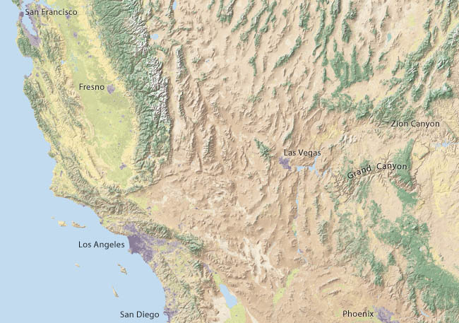
Figure 12. California and the southwestern US depicted with colorized NLCD and shaded relief.

The grouping of colors in the palette attempts to acknowledge the non-hierarchical and interrelated character of the natural world. Although it looks like a conventional legend, further macro level groupings exist within the palette (Figure 11). The highest division is between the natural and human environments. Below this level the overlapping groups contain common colors to infer inter-categorical relationships. For example, the group water consists of woody wetland, herbaceous wetland, and open water, all of which contain blue in varying amounts. The color groupings, which are invisible to the reader, bring natural order to the underlying data and produce more harmonious colors on the final map (Figure 12).

Using NLCD in Adobe Photoshop

Having discussed what to do with NLCD, we now discuss how to do it.

First you will need to obtain NLCD, which is downloadable from two sites maintained by the USGS (see Appendix B for URLs). The USGS Seamless Data Distribution System provides unprojected data (sometimes called the Geographic or Latitude/Longitude projections) for user-selected areas in either ESRI (Environmental Systems Research Institute) compatible GRID format or as a GeoTIF. The USGS also maintains an FTP (File Transfer Protocol) site accessible with a web browser containing individual GeoTIF files for the 48 contiguous states in the Albers Equal-Area Conic projection. The 30-meter-resolution data on both sites is otherwise identical and tend to be large. To produce the map shown in Figure 12, we used a mosaic of NLCD data of the entire contiguous US at 240-meter resolution in the Albers Equal-Area Conic projection, an unpublicized product. The USGS kindly gave us this 19,322-pixel-wide TIF image via FTP in response to an email request sent from the link on their website.

Opening NLCD in GeoTIF format in Photoshop reveals an image with a kaleidoscope of colors similar to those shown in Figure 8. Although NLCD may look like an ordinary RGB (Red-Green-Blue) or CMYK (Cyan-Magenta-Yellow-Black) image, it is in indexed color mode, which is less familiar to many cartographers. The advantage of indexed color mode over, say, RGB color mode, is its compact file size, no larger than an 8-bit grayscale image, and the ability to manage colors, such as those representing land cover categories, via a color table. An indexed color table may contain up to 255 colors.

Going to the drop menu and Image/Mode/Color Table, accesses the Color Table dialog, where you can explore and modify the color palette. Toggling between the presets in the Color Table (Spectrum, Mac OS System, Windows System, etc.) vividly demonstrates how changes to the Color Table can change the appearance of NLCD. Although the jumble of multi-colored squares in the Color Table may look confusing at first, their positions correspond to the numbered categories in the NLCD classification. For example, NLCD category 11 is open water, which occupies the 12th color square in the top row of the Color Table (counting the first square as zero); category 43 evergreen forest occupies the 44th square; and, so forth. If you can count, you can manage indexed NLCD colors in Photoshop.

Changing colors in the Color Table is as simple as clicking on a square and specifying a new color in the Color Picker or using the Eyedropper tool to select a color from any open Photoshop image. Use the Eyedropper tool technique to select natural colors from other maps, scanned art, digital photographs, or any image found on-line. Stuck for a color with which to portray desert southwest shrub? A Google photo search using the keyword “Arizona” will yield a spectrum of choices. Or maybe a snapshot of your golden retriever might contain the ideal color. Hint: you may need to click the okay button to confirm your color table changes before the Eyedropper tool works as expected between uses. Once you have chosen new colors that you like, the modified Color Table is savable and loadable for use with later projects and sessions (Figure 13). The Color Table used in this project is downloadable here.

Figure 13. Using the Color Table in Adobe Photoshop with NLCD in indexed color mode to convert USGS colors (left) to natural colors (right).

Other tips for working with NLCD include:

• If you plan on reprojecting NLCD with GIS or cartographic software (NLCD is formatted to decimal degrees) use data downloaded from the Seamless Data Distribution System. For reprojecting in GIS, GRID (the default) or GeoTIF formats work equally well. After reprojecting is complete, save NLCD in TIF format (with no compression) to bring it into Adobe Photoshop. Should you find yourself with a standard grayscale or RGB image after reprojecting NLCD, in Photoshop going to Image/Mode/Indexed Color allows you to convert the data back to indexed color mode. However, be aware that Photoshop randomly generates new positions for the colors in the Color Table upon returning to indexed color mode. Therefore, it is best to apply the final colors via the Color Table prior to reprojecting NLCD.
  
  
• Indexed color mode images in Photoshop may interpolate incorrectly on screen with a jittery appearance at some zoom levels. If you are not seeing what you expected, zoom in or out until the image appears smoother.
  
  
• When resampling (changing the pixel dimensions) NLCD in Photoshop, it is key to use “nearest neighbor” interpolation to preserve the purity of colors assigned to land cover categories. Using “bicubic” (the Photoshop default) or “bilinear’ interpolation for image resampling and other transformations yields intermediate colors, which do not respond to Color Table manipulations.
  
  
• Photoshop’s functionality is limited in indexed color mode (layers and filters, for example, are disabled). Therefore it is necessary to switch from indexed color mode to RGB or CMYK color modes for the final production of natural-color maps. Do this only after the application of final colors in the Color Table in indexed color mode.
  
  
• As a last step before compositing NLCD with shaded relief to make the final map, apply a slight amount of Gaussian blur (Filter/Blur/Gaussian Blur) to the data. Set the blur radius to 0.5 pixels as a starting point. Applying blur softens the harsh grainy appearance of NLCD, a condition that commonly afflicts images processed with nearest neighbor interpolation. Because making color changes to NLCD with the Color Table is impossible after applying Gaussian blur, as a precaution you should use a duplicate file for this final step. Also, excluding the open water category from blurring will preserve crisp, well-defined shorelines and drainages.

The USGS is currently revising NLCD based on 2001-era Landsat 7 Enhanced Thematic Mapper Plus imagery. Limited areas of the US are now available in the same classification system as the 1992 NLCD just discussed. These upgraded land cover datasets are better able to accommodate mixed spectral signatures across image mosaics and multiple time captures of vegetation, which means that besides being newer, they are more accurate. Perhaps the new NLCD will include Alaska and Hawaii, too.