Tom Patterson
U.S. National Park Service
Harpers Ferry Center
Harpers Ferry, WV 25425-0050
Update - April 2004: With the release of Adobe Photoshop CS (v. 8), which now includes expanded support for 16-bit data, including layering, the DEM manipulation techniques described below are much easier to accomplish. In addition, Mac OSX users can export 16-bit DEMs from Photoshop 7.0 and CS in PGM format readable by Bryce using the free CartaPGM filter developed by Pascal Lamboley and Bernhard Jenny available here.
Introduction
This article discusses the graphical techniques used by the U.S. National Park Service (NPS) in manipulating Digital Elevation Models (DEMs) for the design and production of 3D landscape visualizations. Over the past five years, the NPS has relied increasingly on portraying geographic information through 3D visualizations—static images, animations, and interactive scenes—which are assumed to be more easily understood by casual visitors than more abstract two-dimensional (2D) maps and illustrations in interpreting the natural and cultural resources of the 384 units in the National Park System. The types of 3D visualizations created by the NPS include geologic block diagrams; natural science illustrations, 3D hiking maps, Heinrich Berann-style panoramas, and birds-eye views of cultural sites showing buildings, landscaping, and vegetation set on topographic models.
DEMs—the term is used generically here to describe all varieties of spatially-arranged elevation data, regardless of format—comprise the digital foundation upon which all 3D landscape visualizations are based. Despite the importance of DEMs, cartographers and GIS specialists generally hesitate to manipulate DEMs for enhancing 3D visualizations—in contrast to their willingness to modify vector data routinely to enhance 2D maps. Manipulations to DEMs are usually made only to edit imperfect data, such as systematic banding and discrepancies in matching edges. This hands-off approach to DEMs may have several causes: the lingering belief that DEMs, like the landscapes they represent, are largely immutable; well intentioned respect for maintaining the integrity of data created by others; and unfamiliarity with the necessary software applications and techniques, and the concept of DEM manipulation itself.
Why manipulate DEMs?
Practical reasons abound for manipulating DEMs beyond routine editing of cosmetic data imperfections. As in all cartographic presentation, geographic reality and graphic reality are often at cross purposes. Just as vector data must be simplified to be legible on a 2D map, DEMs must be generalized at reduced scales to avoid creating topography that looks more like a noisy graphical texture than a 3D landscape. This problem can be ameliorated with resolution bumping, a DEM manipulation technique that yields legible small-scale 3D topography in rugged high mountains without sacrificing detail. On the other extreme, small topographic features whose is importance is disproportionate to their size can be given greater emphasis by using selective vertical exaggeration. For example, Puu Oo volcano on the island of Hawaii has a surface area of only 10 hectares but has sheathed 105 square kilometers of Hawaii with lava since it began continually erupting in 1983. With selective vertical exaggeration, Puu Oo could be exaggerated in height and made more discernable next to its dominant neighbor, Mauna Loa, whose mass is greater than any other solitary mountain in the World.
The most dramatic DEM manipulation techniques may be those that depict geologic processes. Starting with a DEM of an existing landscape, the user can either reverse-engineer topography to portray an earlier stage of landscape development or project it into the future. Like virtual modeling clay, DEMs are pliable; they allow users to create an almost unlimited variety of derivative or even entirely new landscapes. The challenge when altering the topographic morphology of DEMs is to do so with the control and precision required for geographic visualization.
Approaches to DEM manipulation
The software used to manipulate DEMs can generally be categorized as either cartographic/GIS and graphic. Although the applications in each category have similarities (such as their underlying algorithms), they are used by entirely different professional cultures to produce different products. GIS applications, as most readers of this text are well aware, appropriately emphasize spatial analysis and accuracy, but the relatively staid 3D graphical capabilities of these applications provide few tools for creatively manipulating DEMs. By contrast, graphical 3D software applications generally contain a plethora of tools, some with real-time interactivity, for manipulating elevation data to create eye-catching special effects. The landscapes yielded by graphical software are used mostly for entertainment (computer games and movie special effects), fine art, and fantasy/science fiction pursuits. Despite these imaginative ends, graphical 3D software tends to have limited DEM import capabilities. Imaginary fractally-generated terrains, some stunningly realistic, are the landscape type of choice (Musgrave 1998). Geographic accuracy, if addressed at all, is often an inconvenient afterthought.
The NPS approach to DEM manipulation bridges the gap between the cartographic/GIS and graphic 3D cultures. 3D visualizations are created with Corel Bryce 4.1, a consumer-oriented, landscape rendering application most famous for its unconventional Kai Krause-inspired graphical user interface (www.corel.com). Because Bryce does not import geo-coded data, helper utilities and a roundabout workaround procedure are used to bring large-format DEMs into the program. However, once the DEM is imported, a powerful suite of 3D special effects exists; the interface is easy-to-use, and the rendering engine yields exceptionally high quality ray-traced output in the form of raster images, animations, or QuickTime Virtual Reality scenes. Although Bryce contains a fascinating terrain editor, which allows DEMs to be manipulated interactively, its cramped interface and inability to edit precisely defined geographic areas limits effectiveness for making professional landscape visualizations (Webster 2001).
Manipulating DEMs in Photoshop
To overcome the shortcomings of Bryce’s terrain editor, the NPS uses Adobe Photoshop (www.adobe.com), the popular image editing application, to manipulate DEMs before importing them into Bryce. Because the NPS already uses Photoshop as a go-between application for importing large format DEMs into Bryce, making DEM manipulations in Photoshop makes practical sense. As raw binary files DEMs can be opened in Photoshop as 16-bit grayscale raster images containing 65,536 levels of height information: with 16-bit vertical resolution you can depict topographic surfaces with near-perfect smoothness. (Contrast this with the 256 elevation levels available in 8-bit DEMs, which often yields topography with stair-stepped surfaces.) BSmooth (www.bsmooth.de), a shareware utility, is then used to convert the 16-bit grayscale DEM from Photoshop format (.psd) to a quadratic-sized file in Portable Grayscale Map format (.pgm), which Bryce can then import.
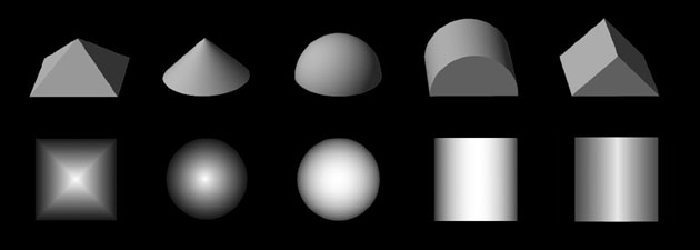
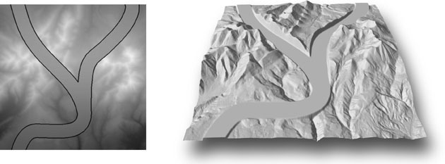
A DEM opened in Photoshop appears as a ghosted grayscale image, similar to an X-ray, with light colored pixels representing high elevations and dark pixels lowlands. Although a grayscale DEM in Photoshop looks nothing like the 3D surface it will eventually become when rendered in Bryce (Figure 1), that it can be seen in pictorial form at all is a huge benefit when making manipulations. Changes can actually be seen, as compared to the original DEM, a text file of numbers that defies visualization.
Notable disadvantages to manipulating DEMs in Photoshop exist. Previewing an edited DEM in 3D involves exporting the DEM from Photoshop, importing it into Bryce, and then rendering the scene—a time consuming process when making repeated subtle edits. More problematic is Photoshop’s limited functionality when using 16-bit images as opposed to “normal” 8-bit images. Most items in the toolbar are disabled as are most filters and the layers palette—16-bit functionality is akin to going back to Photoshop version 1.0.
Despite Photoshop’s diminished 16-bit functionality, it nevertheless contains all the tools needed to manipulate DEMs with the accuracy required for visualization. Clever workarounds, however, are often necessary to perform routine functions. For example, hard-edged and feathered selections can be used on 16-bit DEMs despite the fact that the Magic Wand and Color Range selection tools are disabled in 16-bit mode. Using either of these selection tools requires duplicating a 16-bit DEM file and saving it as an 8-bit proxy to be used only for making selections. The selection boundaries can then be dragged and dropped from the 8-bit file to the 16-bit file. (Hint: temporarily inverting an interior selection allows it to be precisely registered to a corner when dragged into the 16 bit image.) Cartographers can use similar techniques to import selections from rasterized vector geo-data.
Photoshop’s painting tools are also disabled in 16-bit mode. However, the Rubber Stamp tool, which is enabled, is an effective substitute for the Airbrush tool for painting on DEM surfaces. Data can be sampled and cloned between two open 16-bit Photoshop files. By filling a proxy 16-bit file entirely with black or white and then using the rubber stamp with a soft brush and the blending opacity set to a low value, black or white tones can subtly be transferred from the proxy image onto the DEM, lowering or raising elevations respectively.
Photoshop can be used in innumerable ways to manipulate DEMs to enhance 3D landscape visualization. The following emphasize creating static images of 3D landscapes to show some practical techniques used by the NPS:
Generalization
Downsampling means to decrease the resolution or size via the Image Size dialog. Downsampling grayscale DEMs in Photoshop results in more generalized landscape surfaces. For example, a DEM downsampled from 1024 x 1024 pixels to 512 x 512 pixels will have half as much detail as the original and a smoother appearance. In the Preferences dialog, Photoshop offers three interpolation methods for calculating pixel values when downsampling or otherwise transforming images. In general, bicubic interpolation (the default) works best for straight downsampling. If the DEM were also to be rotated, however, "nearest neighbor" interpolation would be a better choice, because this faster interpolation eschews anti aliasing, thus preserving crisp-edged pixels at the margins of the DEM. Regardless of which interpolation method is used, upsampling, the opposite procedure of downsampling, which adds pixels to an image, should generally be avoided. Upsampling only increases the file size (in MB) without increasing the discernable detail.
Alternatively, applying the Gaussian blur filter to a DEM, a method that does not decrease the file size, achieves extremely smooth generalization. The smoothing effects of Gaussian blur filtering behave differently than downsampling; experimentation is required to achieve comparable levels of generalization between the two techniques.
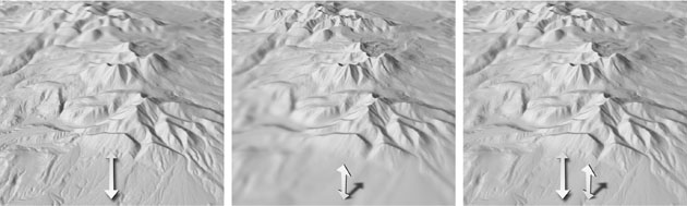
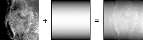
Although generalization is most often applied globally throughout a DEM, it can also be applied in graduated amounts to achieve subtle visual effects. For example, increasing generalization (thereby decreasing visible detail) from foreground to background on a DEM creates the optical illusion of depth when it is viewed in 3D (Figure 2). Foreground to background generalization also hastens rendering time, an important consideration when creating interactive environments (Moore 1999). Graduated generalization can also be applied to the vertical axis of a DEM, creating scenes with more visible detail at higher elevations than at lower elevations. This technique mimics the aerial perspective effect, a visualization technique pioneered by Eduard Imhof, which accounts for the veiling effects of atmospheric haze. When aerial perspective is employed, highlands, which are theoretically closer to the viewer, are depicted with greater detail and contrast than the lowlands further away, enhancing three dimensionality (Imhof 1982).
Finally, greater amounts of resolution can be applied selectively to small but otherwise important topographic features on a DEM, such as Puu Oo, Hawaii mentioned earlier. Detailed objects tend to attract the viewer’s attention more readily than generalized objects (Garfield 1970), a phenomenon that can be exploited beneficially for 3D landscape visualization.
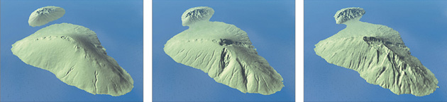
Resolution bumping is a generalization technique for manipulating GTOPO30 and other small-scale DEMs. The technique alters digital elevation surfaces so that rugged, high mountains are more legible and look more natural as compared to unmodified data (Figure 3).
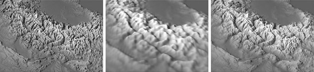
Downsampling GTOPO30 data to a sparser resolution alleviates the problems outlined above. Generalized data is better for depicting patterns within mountain ranges and is more tolerant of vertical exaggeration. Downsampling elevation data, however, introduces new problems that are arguably worse than the now corrected original problems. Knife-edged mountain ridges appear excessively rounded, like the vacuum-formed plastic relief maps used in schools, and simplified valley bottoms are prone to misregistration with drainages.
The idea behind resolution bumping is simple: merging low-resolution and high-resolution GTOPO30 data of the same area produces hybrid data that combine the best characteristics and minimize the problems found in the originals. Two copies of a GTOPO30 file are used, one high resolution and the other downsampled to a lower resolution. These files can then be blended in Photoshop by a proportional amount that is controlled by the user. This technique yields a new grayscale DEM that, if merged in the right proportions, combines the readability of the downsampled data with all the detail one expects to find in mountainous terrain—without the graphical noise. Resolution bumping in effect "bumps" or etches a suggestion of topographical detail onto generalized topographic surfaces. The resolution-bumped data creates an elevated base in mountainous regions, upon which individual mountains, with diminished vertical scaling, project upwards (Patterson 2001).
Height manipulation
Lightening or darkening a DEM with Photoshop’s image adjustment tools (levels, curves, brightness/contrast) raises or lowers surfaces respectively when the DEM is later rendered in 3D. This technique can be used to modify vertical exaggeration globally over an entire DEM or, more interestingly, for selected topographic features. For example, a mountain hosting a ski area could be exaggerated in height above its surroundings (for ski area maps, bigger is better) by using the Lasso tool to draw a selection boundary with a feathered edge around the mountain and lightening the area within the space.
Going one step further, to apply lightening and darkening within selections can create simple topographic features. A volcanic cinder cone can be created by drawing a circular selection with a feathered edge (again with the Lasso tool) and lightening the area within, forming a cone-shaped hill when the DEM is extruded in 3D. Drawing the circular selection with a slightly irregular shape avoids excessive symmetry and gives the cone a more realistic appearance. Lastly, by contracting the initial circular selection by several pixels and applying a smaller amount of darkening, the summit is depressed (see Figure 7, left image).
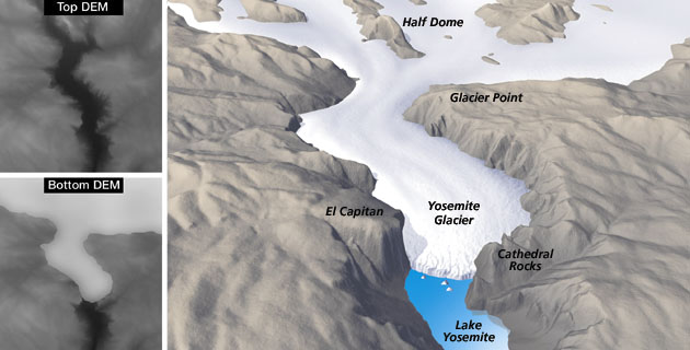
Glaciers can be depicted by manipulating elevation on a duplicated DEM, positioned precisely below the original unaltered DEM in Bryce. In Photoshop, on the bottom DEM an imported selection boundary representing the glacier’s extent is drawn or imported and filled with lighter pixels. Using a feathered selection boundary creates a domed effect when the glacier is extruded in Bryce. By increasing the bottom DEM’s vertical exaggeration and lowering its position in Bryce, the virtual glacier will protrude through the top DEM, neatly intersecting the valley walls (Figure 4).
Taking elevation manipulations to the extreme, you can apply solid black on a DEM to form block diagrams and cut-away views. Black represents the lowest elevation value. When applied to a selected portion of a grayscale DEM it flattens and lowers the topography to base level—the digital equivalent of a peneplain. The bottommost elevation data can then be clipped from a DEM when rendered in 3D. This technique allows selected chunks of a DEM to be cut away, making cross-sectional views or revealing hidden features beneath the surface (Figure 5).

Elevation flattening
The Gaussian blur filter is useful for more than generalizing DEMs. The filter works by filtering pixels (elevations) through a mathematical “soft” lens controlled by a radius slider, which removes detail. When the radius is small, the DEM is merely smoothed; when the radius is excessive and/or applied repeatedly, the DEM flattens. Gaussian blur flattening, when applied to imported selection boundaries, yields benefits. For example, land/water boundaries on DEMs often do not match the same boundaries on imagery or vector linework. This creates unsightly misregistration near the shorelines when these data are later draped on DEMs. Editing the DEM solves the problem. By importing a selection of water bodies taken from the geo-imagery or rasterized vectors (using the drag-and-drop technique described previously) and applying maximum Gaussian blur, water body surfaces on the DEM become perfectly flat at their respective elevations in concert with the draped imagery. The drawback to this technique is the occasional obliteration of distinctive topography immediately bounding water bodies.
Gaussian blur used in moderate amounts has other uses. Applied to a selected area on a slope, elevation-averaging produces terraces uncannily similar to those created by actual earth-moving equipment. This is a useful technique on large-scale DEMs for depicting level areas around buildings. Moreover, moderate Gaussian blur applied to road selections removes excess height data from elevated protuberances and adds data to bisected valleys, creating virtual road cuts and fills (Figure 6).
Edits may be made to DEMs by painting directly on their surfaces (using the Rubber Stamp tool as a substitute for the Airbrush tool on 16-bit DEMs). DEM painting requires manual skills similar to those used in traditional illustration and produces topography with a similar organic appearance. Painting on DEMs is hampered by the disconnect between the appearance of the 2D grayscale DEM, the item that is painted, and 3D model it will eventually become (see Figure 1). The problem is especially acute when painting subtle tones that can be difficult to see on the monochromatic surface of the DEM. Nevertheless, with practice the user can learn to paint DEMs effectively in Photoshop for depicting geological phenomena. For instance, to produce earthquake fissures and glacial crevasses simply draw a network of thin dark lines with tapered ends—an unsteady hand is, for once, a benefit. Stream erosion is another application. Sinuous dark tones applied with multiple light brush strokes, moving in an uphill direction, mimic the growth of drainage basins over time. By using progressively larger brush sizes with soft edges, drainage basins expand in volume to simulate natural erosion (Figure 7).

In describing hypothetical former and future landscapes, geology texts often make comparisons to analogous present-day landscapes. This concept can be applied to making geologic visualizations by cloning topography from one DEM to another in a technique known as topographic substitution. Providing that the user obtains appropriate DEMs, topographic substitution is easier than DEM painting, and, because it is based on actual DEMs, it looks convincingly realistic.
Topographic substitution is accomplished with the Rubber Stamp tool by cloning data between simultaneously opened 16-bit DEMs. All of Photoshop’s blending modes can be used at varying opacities. The possibilities for mixing and matching topography to create hybrid landscapes are nearly unlimited. For example, a depiction of the primordial landscape of Virginia, the state where I now live, could be made by combining a strato volcano, cloned from a present-day DEM of Alaska, onto a DEM of the bayou country of Louisiana. Other applications could include showing the weather-worn Appalachian Mountains in their former lofty glory by grafting a DEM of today’s Rockies on top of the Appalachians; merging the Kaibab and Coconino Plateaus together to in fill the Grand Canyon; or placing Mt. Adams on top of Crater Lake to depict ancient Mt. Mazama before it erupted and imploded to form today’s caldera lake (Figure 9).

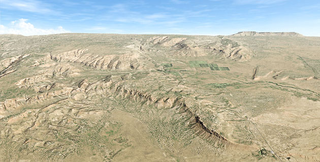
The projection plane of DEMs—the digital datum upon which 3D terrain projects upwards—is flat. Using flat-world terrain models, however, can impede 3D visualization. On low-elevation views the landscape looks most dramatically realistic when the horizon is visible, but tall topographic features in the foreground often obscure important features deeper in the scene. Moreover, even if the entire scene were visible, the oblique viewing angle renders surface information difficult or impossible to read. Raising the viewing elevation usually solves these problems, but then the landscape looks too much like a conventional map, eliminating the advantages of 3D visualization.
A better solution is to emulate the view as seen from an airplane. From high above the Earth the horizon is always visible, yet when you shift your eyes downward the view gradually becomes less oblique and more planimetric (Figure 10). This effect can be brought to 3D landscape visualization by adding convex curvature to the DEM and tilting the scene toward the viewer (Figure 11). The end result is a 3D scene that combines the best of both worlds: the foreground and middleground (where the important information resides) appear map-like, while the background appears realistic, complete with a horizon and sky (Patterson 2000).
Using Photoshop to manipulate DEMs—a purpose for which the software is not specifically intended—has enabled the NPS to enhance 3D visualizations economically, ultimately benefiting park visitors by presenting landscapes and geo-spatial information in a more comprehensible manner.
This review of techniques does not give detailed step-by-step instructions because space is limited and software evolves so fast that they would be out of date soon. The Photoshop techniques used by the NPS for manipulating DEMs will undoubtedly be superseded by dedicated terrain applications that allow geo-data to be edited interactively. One such promising application is Leveller (www.daylongraphics.com), which can import and export a wide range of DEM file formats, import selection boundaries, apply Photoshop-like filtering, and allow painting and cloning on DEM surfaces with real-time 3D feedback. Another promising application is World Construction Set (WCS), a professional, albeit difficult to learn, 3D landscape application that uses geo-coded data to render photo-realistic scenes complete with user-defined ecosystems and vegetation (www.3dnature.com). Using DEMs loaded into its database, WCS calculates varying amounts of topographic detail on-the-fly to depict background areas with less detail than the foreground, enhancing 3D depth and speeding rendering times. In addition, WCS uses imported vectors, called Terraffectors (tm), to etch drainages onto DEM surfaces, grade roads, and selectively modify vertical exaggeration.
If Leveller and World Construction Set are any indication, the future of 3D landscape visualization looks bright. And as the cartographic and GIS communities begin to use these new tools, the techniques discussed here will, I hope, serve as a benchmark for further visual exploration.
Literature
Garfield, Terry. 1970. The Panorama and Reliefkarte of Heinrich Berann. Bulletin of the Society of University Cartographers. Vol. 4, No. 2, Liverpool, pp. 52-61.
Imhof, Eduard. 1982. Cartographic Relief Presentation. H.J. Steward (edited by), Walter de
Gruyter, Berlin & New York, pp. 389.
Moore, Kate. 1999. VRML and Java for Interactive 3D Cartography. Multimedia Cartography. Springer-Verlag, Berlin, W. Cartwright, G. Gartner, M. Peterson (edited by), pp. 205-216.
Musgrave, Kenton. 1998. Procedural Fractal Terrains. Textures and Modeling: A Procedural Approach. 2nd ed. Academic Press, Cambridge, MA, D.S. Ebert (edited by), pp. 450.
Patterson, Tom. 2000. A View from on High: Heinrich Berann's Panoramas and Landscape Visualization Techniques for the U.S. National Park Service. Cartographic Perspectives. No. 36, Spring 2000, pp. 38-65.
Patterson, Tom. 2001. Retro Relief Shading with Adobe Photoshop and a Wacom Tablet. www.nps.gov/carto/silvretta/retro/index.html.
Patterson, Tom. 2001. Resolution bumping GTOPO30 in Photoshop: How to make high mountains more legible. www.nps.gov/carto/silvretta/bumping/bumping.html.
Webster, Garrick. 2001. Bryce Age. 3D World. Issue 12, Future Publishing, Ltd., Bath, U.K., pp. 48-50.
Software
Adobe Photoshop. www.adobe.com
Corel Bryce. www.corel.com
Leveller. www.daylongraphics.com
MacDEM. www.treeswallow.com
World Construction Set. www.3dnature.com